Commands frame:/loopy_belief_propagation
Message passing to infer state probabilities.
POST /v1/commands/
GET /v1/commands/:id
Request
Route
POST /v1/commands/
Body
| name: | frame:/loopy_belief_propagation |
|---|---|
| arguments: | frame : <bound method AtkEntityType.__name__ of <trustedanalytics.rest.jsonschema.AtkEntityType object at 0x7f9e686f3fd0>>
src_col_name : unicode
dest_col_name : unicode
weight_col_name : unicode
src_label_col_name : unicode
result_col_name : unicode (default=None)
ignore_vertex_type : bool (default=None)
max_iterations : int32 (default=None)
convergence_threshold : float32 (default=None)
anchor_threshold : float64 (default=None)
smoothing : float32 (default=None)
max_product : bool (default=None)
power : float32 (default=None)
|
Headers
Authorization: test_api_key_1
Content-type: application/json
Description
Loopy belief propagation on Markov Random Fields (MRF). Belief Propagation (BP) was originally designed for acyclic graphical models, then it was found that the BP algorithm can be used in general graphs. The algorithm is then sometimes called “Loopy” Belief Propagation (LBP), because graphs typically contain cycles, or loops.
Loopy Belief Propagation (LBP)
Loopy Belief Propagation (LBP) is a message passing algorithm for inferring state probabilities, given a graph and a set of noisy initial estimates. The LBP implementation assumes that the joint distribution of the data is given by a Boltzmann distribution.
For more information about LBP, see: “K. Murphy, Y. Weiss, and M. Jordan, Loopy-belief Propagation for Approximate Inference: An Empirical Study, UAI 1999.”
LBP has a wide range of applications in structured prediction, such as low-level vision and influence spread in social networks, where we have prior noisy predictions for a large set of random variables and a graph encoding relationships between those variables.
The algorithm performs approximate inference on an undirected graph of hidden variables, where each variable is represented as a node, and each edge encodes relations to its neighbors. Initially, a prior noisy estimate of state probabilities is given to each node, then the algorithm infers the posterior distribution of each node by propagating and collecting messages to and from its neighbors and updating the beliefs.
In graphs containing loops, convergence is not guaranteed, though LBP has demonstrated empirical success in many areas and in practice often converges close to the true joint probability distribution.
Discrete Loopy Belief Propagation
LBP is typically considered a semi-supervised machine learning algorithm as
- there is typically no ground truth observation of states
- the algorithm is primarily concerned with estimating a joint probability function rather than with classification or point prediction.
The standard (discrete) LBP algorithm requires a set of probability thresholds
to be considered a classifier.
Nonetheless, the discrete LBP algorithm allows Test/Train/Validate splits of
the data and the algorithm will treat “Train” observations
differently from “Test” and “Validate” observations.
Vertices labeled with “Test” or “Validate” will be treated as though they have
uninformative (uniform) priors and are
allowed to receive messages, but not send messages.
This simulates a “scoring scenario” in which a new observation is added to a
graph containing fully trained LBP posteriors, the new vertex is scored based
on received messages, but the full LBP algorithm is not repeated in full.
This behavior can be turned off by setting the ignore_vertex_type parameter
to True.
When ignore_vertex_type=True, all nodes will be considered “Train”
regardless of their sample type designation.
The Gaussian (continuous) version of LBP does not allow Train/Test/Validate
splits.
The standard LBP algorithm included with the toolkit assumes an ordinal and
cardinal set of discrete states.
For notational convenience, we’ll denote the value of state  as
as
 , and the prior probability of state
as
, and the prior probability of state
as  .
.
Each node sends out initial messages of the form:
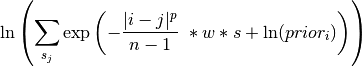
Where
 is the weight between the messages destination and origin vertices
 is the smoothing parameter
 is the power parameter
 is the number of states
The larger the weight between two nodes, or the higher the smoothing parameter,
the more neighboring vertices are assumed to “agree” on states.
We represent messages as sums of log probabilities rather than products
of non-logged probabilities which makes it easier to subtract messages in the
future steps of the algorithm.
Also note that the states are cardinal in the sense that the “pull” of state
on state  depends on the distance between and
.
The power parameter intensifies the rate at which the pull of distant states
drops off.
depends on the distance between and
.
The power parameter intensifies the rate at which the pull of distant states
drops off.
In order for the algorithm to work properly, all edges of the graph must be
bidirectional.
In other words, messages need to be able to flow in both directions across
every edge.
Bidirectional edges can be enforced during graph building, but the LBP function
provides an option to do an initial check for bidirectionality using the
bidirectional_check=True option.
If not all the edges of the graph are bidirectional, the algorithm will return
an error.
Look at a case where a node has two states, 0 and 1.
The 0 state has a prior probability of 0.9 and the 1 state has a prior
probability of 0.2.
The states have uniform weights of 1, power of 1 and a smoothing parameter of 2.
The nodes initial message would be ![\textstyle \left [ \ln \left ( 0.2 \
+ 0.8 e ^{-2} \right ), \ln \left ( 0.8 + 0.2 e ^{-2} \right ) \right ]](../../../f_images/math/3079aadf373db4dad93b9940cc3d3c1e0a50b0a2.png) ,
which gets sent to each of that node’s neighbors.
Note that messages will typically not be proper probability distributions,
hence each message is normalized so that the probability of all states sum to 1
before being sent out.
For simplicity of discussion, we will consider all messages as normalized
messages.
,
which gets sent to each of that node’s neighbors.
Note that messages will typically not be proper probability distributions,
hence each message is normalized so that the probability of all states sum to 1
before being sent out.
For simplicity of discussion, we will consider all messages as normalized
messages.
After nodes have sent out their initial messages, they then update their
beliefs based on messages that they have received from their neighbors,
denoted by the set  .
.
Updated Posterior Beliefs:
![\ln (newbelief) = \propto \exp \left [ \ln (prior) + \sum_k message _{k} \
\right ]](../../../f_images/math/2698aa55e8a9d5cc8a66eb4844aaefa35e7abb2d.png)
Note that the messages in the above equation are still in log form. Nodes then send out new messages which take the same form as their initial messages, with updated beliefs in place of priors and subtracting out the information previously received from the new message’s recipient. The recipient’s prior message is subtracted out to prevent feedback loops of nodes “learning” from themselves.

In updating beliefs, new beliefs tend to be most influenced by the largest
message.
Setting the max_product option to “True” ignores all incoming messages
other than the strongest signal.
Doing this results in approximate solutions, but requires significantly less
memory and run-time than the more exact computation.
Users should consider this option when processing power is a constraint and
approximate solutions to LBP will be sufficient.
This process of updating and message passing continues until the convergence
criteria is met or the maximum number of supersteps is
reached without converging.
A node is said to converge if the total change in its distribution (the sum of
absolute value changes in state probabilities) is less than
the convergence_threshold parameter.
Convergence is a local phenomenon; not all nodes will converge at the same
time.
It is also possible for some (most) nodes to converge and others to never
converge.
The algorithm requires all nodes to converge before declaring that the
algorithm has converged overall.
If this condition is not met, the algorithm will continue up to the maximum
number of supersteps.
See: http://en.wikipedia.org/wiki/Belief_propagation.
Response
Status
200 OK
Body
Returns information about the command. See the Response Body for Get Command here below. It is the same.